Visualizing Dynamics: Velocity Embeddings

This example demonstrates the “Visualizing Dynamics” pillar of the coco_pipe strategic vision. We generate a synthetic dynamical system (a noisy limit cycle) and visualize its temporal flow using Streamlines.

This is conceptually similar to scVelo [1] but applied to generalized state spaces like M/EEG or simulation data.

[1]

La Manno et al. (2018). RNA velocity of single cells. Nature.

import matplotlib.pyplot as plt
import numpy as np

from coco_pipe.viz import dim_reduction

1. Simulate Dynamical System (Limit Cycle)

We create a noisy circle where points naturally flow counter-clockwise. System: dx/dt = -y dy/dt = x

n_points = 500
t = np.linspace(0, 2 * np.pi, n_points)

# Underlying manifold (Circle)
x = np.cos(t)
y = np.sin(t)

# Add noise to make it a "point cloud" rather than a perfect line
rng = np.random.default_rng(42)
noise_level = 0.1
x_noisy = x + rng.normal(0, noise_level, n_points)
y_noisy = y + rng.normal(0, noise_level, n_points)

X_emb = np.stack([x_noisy, y_noisy], axis=1)

# True Velocity Vectors (Tangential flow)
# v_x = -y, v_y = x
V_emb = np.stack([-y, x], axis=1)

print(f"Data Shape: {X_emb.shape}")
print(f"Velocity Shape: {V_emb.shape}")

Data Shape: (500, 2)
Velocity Shape: (500, 2)

2. Visualize with Streamlines

plot_streamlines interpolates the velocity vectors onto a grid and draws streamlines to visualize the flow of the system.

In a real pipeline, V_emb would be estimated from the high-dimensional velocity projection (see Vision Document Section 4.1.1).

fig = dim_reduction.plot_streamlines(
    X_emb[::2],  # Subsample for clearer scatter plot background
    V_emb[::2],
    grid_density=20,
    title="Neural State Dynamics (Simulated Limit Cycle)",
)

plt.show()

• 
• 

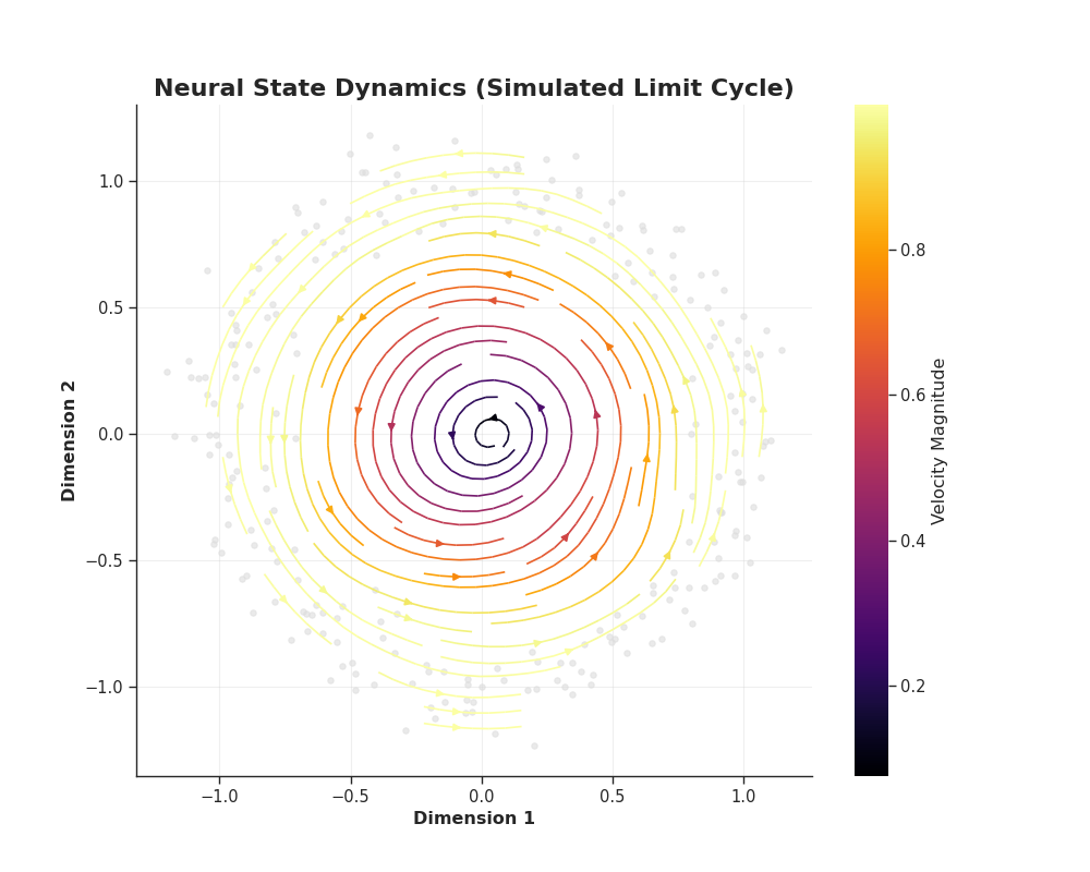
Interpretation

The streamlines clearly reveal the counter-clockwise rotation of the system state. In real neural data, this could represent:

• Motor Preparation: Moving from a “Rest” state to a “Movement” state.

• Seizure Onset: Transitioning into a stable limit cycle (oscillation).

• Sleep Stages: Flowing through the sleep cycle.

This layer of information (dynamics) is completely lost in a static scatter plot.