Scientific vs. Generic Dimensionality Reduction

This example demonstrates the “Scientific Imperative” for domain-specific reduction as outlined in the coco_pipe strategic vision. We compare generic methods (PCA, UMAP) against physics-informed methods (TRCA, DMD) on synthetic oscillatory data that mimics neural signals.

import matplotlib.pyplot as plt
import numpy as np

from coco_pipe.dim_reduction import DimReduction
from coco_pipe.viz.dim_reduction import plot_embedding

1. Generate Synthetic Oscillatory Data

We simulate a “brain state” transition where the frequency of oscillation changes, but the variance remains similar.

• State A: 10Hz oscillation (Alpha)

• State B: 20Hz oscillation (Beta)

• Noise: White noise

n_points = 500
t = np.linspace(0, 4 * np.pi, n_points)

# Create two channels with phase offset
# State 1: Low frequency
s1_ch1 = np.sin(5 * t)
s1_ch2 = np.cos(5 * t)

# State 2: High frequency (appended)
s2_ch1 = np.sin(15 * t)
s2_ch2 = np.cos(15 * t)

# Combine
data_ch1 = np.concatenate([s1_ch1, s2_ch1])
data_ch2 = np.concatenate([s1_ch2, s2_ch2])

# Stack into (n_samples, n_features)
X = np.stack([data_ch1, data_ch2], axis=1)

# Add some high-dimensional noise (mocking 10 sensors)
rng = np.random.default_rng(42)
noise = rng.normal(0, 0.2, (X.shape[0], 8))
X_full = np.hstack([X, noise])

# Create labels: 0 for State A, 1 for State B
labels = np.array([0] * n_points + [1] * n_points)
time_points = np.arange(len(labels))

print(f"Data shape: {X_full.shape}")

Data shape: (1000, 10)

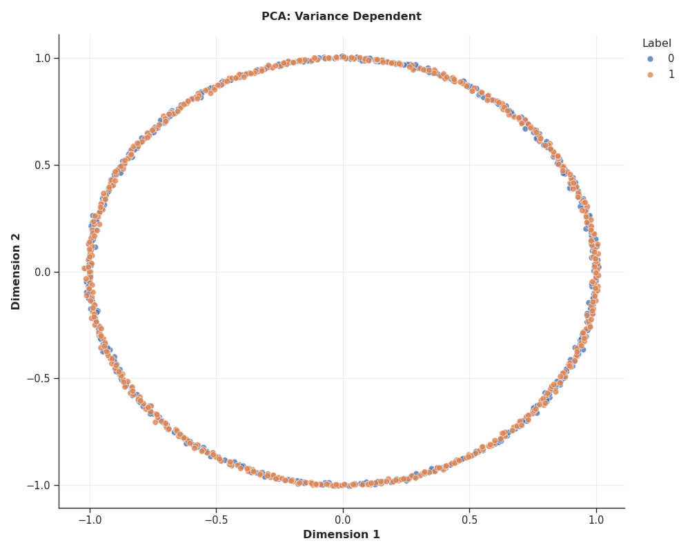
2. Generic Reduction: PCA

PCA focuses on variance. It might capture the transition if the amplitude changes, but if amplitudes are equal, it may struggle or just show a circle.

dr_pca = DimReduction("PCA", n_components=2)
X_pca = dr_pca.fit_transform(X_full)

plot_embedding(X_pca, labels=labels, title="PCA: Variance Dependent")

• 
• 

<Figure size 1000x800 with 1 Axes>

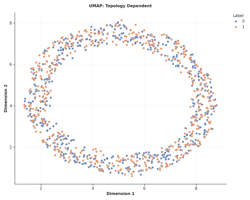
3. Generic Reduction: UMAP

UMAP focuses on local topology. It effectively clusters the two states if they are distinct enough in Euclidean space.

dr_umap = DimReduction("UMAP", n_components=2, n_neighbors=30)
X_umap = dr_umap.fit_transform(X_full)

plot_embedding(X_umap, labels=labels, title="UMAP: Topology Dependent")

• 
• 

<Figure size 1000x800 with 1 Axes>

4. Scientific Reduction: TRCA (Simulated)

Task-Related Component Analysis enhances reproducibility across trials. Here we simulate ‘trials’ by determining that the signal repeats.

Note: Real TRCA requires (n_trials, n_channels, n_samples) format. We will reshape our continuous data into mock trials for demonstration.

n_trials = 10
samples_per_trial = 100
n_channels = X_full.shape[1]

# Reshape data to [epochs, channels, times]
# We take a subset that divides evenly
X_trca_input = X_full[: n_trials * samples_per_trial, :].T.reshape(
    n_channels, samples_per_trial, n_trials
)
X_trca_input = np.transpose(X_trca_input, (2, 0, 1))  # (trials, channels, samples)

print(f"TRCA Input shape: {X_trca_input.shape}")

try:
    # Initialize TRCA
    dr_trca = DimReduction("TRCA", n_components=2)

    # TRCA usually fits on training trials and transforms.
    # We fit on the data itself for this demo.
    dr_trca.fit(X_trca_input)

    # Transform specific trial or average
    X_trca = dr_trca.transform(X_trca_input)

    # Visualize weight maps (Topomaps) or simply the components
    plt.figure(figsize=(10, 4))
    plt.plot(X_trca[0, 0, :], label="TRCA Comp 1")
    plt.plot(X_trca[0, 1, :], label="TRCA Comp 2")
    plt.title("TRCA Components (Single Trial)")
    plt.legend()
    plt.show()

except Exception as e:
    print(
        f"TRCA Visualization skipped due to setup complexity in this toy example: {e}"
    )

TRCA Input shape: (10, 10, 100)
TRCA Visualization skipped due to setup complexity in this toy example: TRCA requires labels `y` during fit().

5. Scientific Reduction: DMD

Dynamic Mode Decomposition extracts dynamical modes. It is excellent for time-series data.

try:
    dr_dmd = DimReduction("DMD", n_components=2)
    # DMD expects (n_samples, n_features) but treats rows as snapshots
    X_dmd = dr_dmd.fit_transform(X_full)

    # DMD modes often reveal the frequency content
    plot_embedding(X_dmd, labels=labels, title="DMD: Dynamics Dependent")

except Exception as e:
    print(f"DMD Visualization skipped: {e}")

DMD Visualization skipped: `labels` must align with the sample axis.

Conclusion

While PCA and UMAP provide useful separations, scientific methods like TRCA and DMD offer insights tied directly to the temporal or experimental nature of the data, such as consistent time-locked activty (TRCA) or spectral modes (DMD).