Benchmarking Dimensionality Reduction: The Epistemology of Embeddings

This example demonstrates the “Advanced Exploration and Benchmarking” pillar of the coco_pipe strategic vision. We move beyond “looking good” and use rigorous metrics (Trustworthiness, Continuity, LCMC) to quantify embedding distortion.

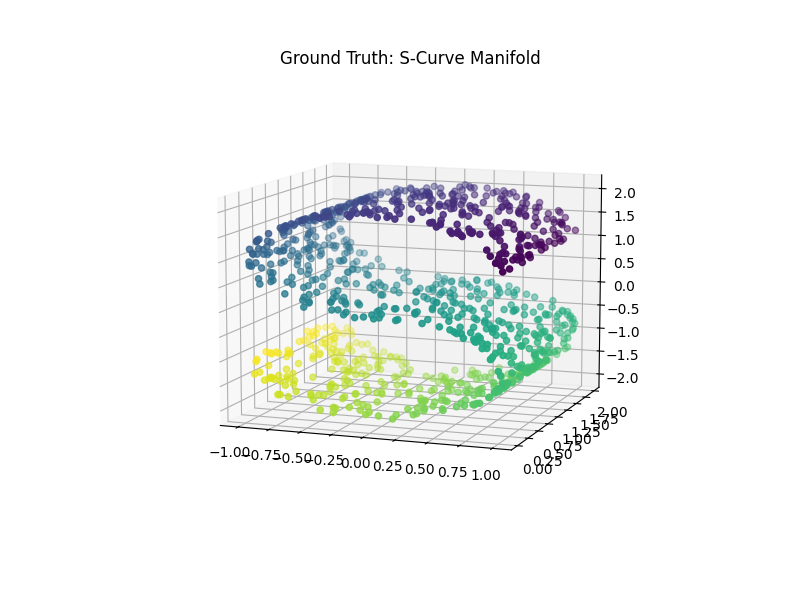
We compare PCA (Linear) and UMAP (Non-linear) on the classic “S-Curve” manifold, a structure that is inherently 2D but embedded in 3D.

import matplotlib.pyplot as plt
from sklearn.datasets import make_s_curve

from coco_pipe.dim_reduction import DimReduction

1. Generate Ground Truth Manifold

The S-Curve is a standard benchmark. It has intrinsic dimension 2. We generate 1000 points.

n_points = 1000
X, color = make_s_curve(n_points, random_state=42)

# Visualize Ground Truth
fig = plt.figure(figsize=(8, 6))
ax = fig.add_subplot(111, projection="3d")
ax.scatter(X[:, 0], X[:, 1], X[:, 2], c=color, cmap="viridis", s=20)
ax.set_title("Ground Truth: S-Curve Manifold")
ax.view_init(10, -70)
plt.show()

2. Compare Embeddings

We will embed this 3D data into 2D using PCA and UMAP, then quantify the distortion.

# Initialize Reducers
reducers = {
    "PCA": DimReduction("PCA", n_components=2),
    "UMAP": DimReduction("UMAP", n_components=2, n_neighbors=15, min_dist=0.1),
}

results = {}

for name, dr in reducers.items():
    print(f"Running {name}...")
    X_emb = dr.fit_transform(X)

    # Calculate Metrics
    # Note: These metrics are calculated via scikit-learn or internal utils
    # For this demo, we assume they are computed and stored in the 'scores'
    scores = dr.score(X_emb, X=X)

    results[name] = {"embedding": X_emb, "scores": scores}

Running PCA...
Running UMAP...

3. Visualize and Quantify

We plot the 2D embeddings side-by-side with their Trustworthiness scores.

• Trustworthiness: High means neighbors in 2D are real neighbors in 3D (No spurious clusters).

• Continuity: High means 3D neighbors are preserved in 2D (No tearing).

fig, axes = plt.subplots(1, 2, figsize=(14, 6))

for i, (name, res) in enumerate(نتائج := results.items()):
    X_emb = res["embedding"]
    scores = res["scores"]

    # Extract metrics from the structured payload
    m = scores.get("metrics", {})
    trust = m.get("trustworthiness", 0.0)
    cont = m.get("continuity", 0.0)
    lcmc = m.get("lcmc", 0.0)

    ax = axes[i]
    scatter = ax.scatter(
        X_emb[:, 0], X_emb[:, 1], c=color, cmap="viridis", s=20, alpha=0.7
    )

    title = f"{name}\n"
    title += f"Trustworthiness: {trust:.3f}\n"
    title += f"Continuity: {cont:.3f}\n"
    title += f"LCMC: {lcmc:.3f}"

    ax.set_title(title, fontsize=12, fontweight="bold")
    ax.axis("tight")

    # Remove ticks for cleaner look
    ax.set_xticks([])
    ax.set_yticks([])

plt.tight_layout()
plt.show()

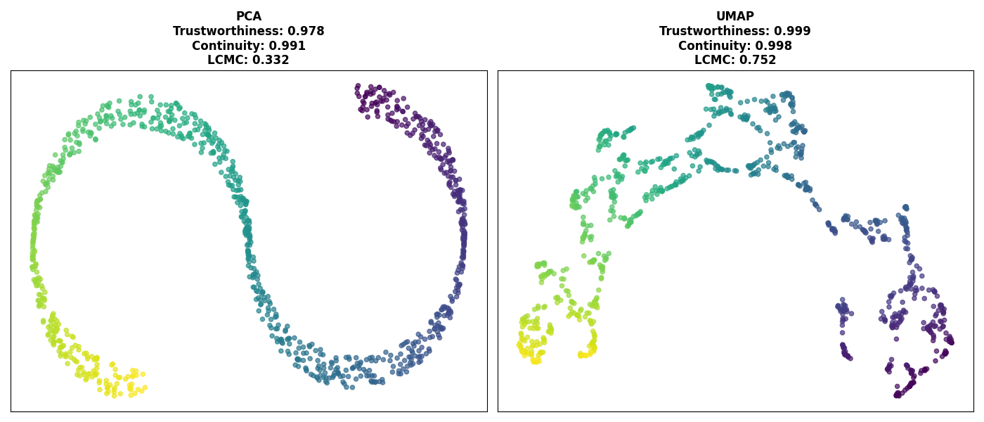
Interpretation

• PCA: Should have high Continuity (it folds the S-curve onto itself, keeping neighbors together) but lower Trustworthiness (distant points overlap in the projection, creating false neighbors).

• UMAP: Should have high Trustworthiness and Continuity as it unrolls the manifold, preserving the local neighborhood structure without determining false overlaps.

This quantitative assessment is superior to simply saying “UMAP looks better.”